MapReduce - Simplified Data Processing on Large Clusters

번역
주석

Jeff Dean과 Sanjay Ghemawat의 2004년 논문.

번역

Jeffrey Dean and Sanjay Ghemawat

jeff @ google.com, sanjay @ google.com

Google, Inc.

Abstract

초록

MapReduce is a programming model and an associated implementation for processing and generating large data sets. Users specify a map function that processes a key/value pair to generate a set of intermediate key/value pairs, and a reduce function that merges all intermediate values associated with the same intermediate key. Many real world tasks are expressible in this model, as shown in the paper.

MapReduce는 대규모 데이터 세트를 처리하고 생성하기 위한 프로그래밍 모델과 그에 대한 구현체입니다. 사용자는 키/값 쌍을 처리하여 중간 키/값 쌍의 집합을 생성하는 map 함수와, 동일한 중간 키에 연관된 모든 중간 값들을 병합하는 reduce 함수를 지정합니다. 이 논문에서는 이 모델로 표현할 수 있는 많은 실제적인 작업들을 보여줍니다.

Programs written in this functional style are automatically parallelized and executed on a large cluster of commodity machines. The run-time system takes care of the details of partitioning the input data, scheduling the program’s execution across a set of machines, handling machine failures, and managing the required inter-machine communication. This allows programmers without any experience with parallel and distributed systems to easily utilize the resources of a large distributed system.

이런 식의 함수형 스타일로 작성된 프로그램은 자동으로 병렬화되어, 대규모의 표준 사양의 머신들로 구성된 클러스터에서 실행됩니다. 런타임 시스템은 입력 데이터를 분할하고, 여러 머신에 걸쳐 프로그램 실행을 스케쥴링하고, 머신의 실패를 처리하고, 필수적인 머신 간의 통신을 관리하는 세부 사항들을 처리합니다. 이를 통해 병렬 및 분산 시스템에 대한 경험이 전혀 없는 프로그래머들도 쉽게 대규모 분산 시스템 자원을 활용할 수 있습니다.

Our implementation of MapReduce runs on a large cluster of commodity machines and is highly scalable: a typical MapReduce computation processes many terabytes of data on thousands of machines. Programmers find the system easy to use: hundreds of MapReduce programs have been implemented and upwards of one thousand MapReduce jobs are executed on Google’s clusters every day.

우리의 MapReduce 구현체는 대규모의 표준화된 머신들로 구성된 클러스터에서 실행되며, 매우 확장성이 높습니다: 일반적인 MapReduce 계산은 수천 대의 머신 위에서 수 테라바이트의 데이터를 처리합니다. 프로그래머들은 이 시스템을 쉽게 사용할 수 있습니다: 수백 개의 MapReduce 프로그램이 이미 구현되었으며, 하루에 1,000개가 넘는 MapReduce 작업이 Google의 클러스터에서 실행되고 있습니다.

1 Introduction

서론

Over the past five years, the authors and many others at Google have implemented hundreds of special-purpose computations that process large amounts of raw data, such as crawled documents, web request logs, etc., to compute various kinds of derived data, such as inverted indices, various representations of the graph structure of web documents, summaries of the number of pages crawled per host, the set of most frequent queries in a given day, etc. Most such computations are conceptually straightforward. However, the input data is usually large and the computations have to be distributed across hundreds or thousands of machines in order to finish in a reasonable amount of time. The issues of how to parallelize the computation, distribute the data, and handle failures conspire to obscure the original simple computation with large amounts of complex code to deal with these issues.

최근 5년간 저자를 비롯한 Google의 많은 직원들은, 크롤링된 문서, 웹 리퀘스트 로그와 같은 대량의 원시 데이터를 처리하는 수백 개의 특수 목적 계산을 구현하여, 역방향 인덱스, 웹 문서의 그래프 구조 표현, 호스트에서 가장 빈번하게 크롤링되는 페이지의 수 요약, 특정한 날에 가장 빈도 높은 쿼리의 집합과 같은 다양한 종류의 파생 데이터를 계산해왔습니다.

이런 계산들은 대부분 개념상으로는 간단하지만, 일반적으로 입력 데이터가 매우 큰 규모이기 때문에 합리적인 시간 내에 계산을 완료하려면 수백에서 수천 대의 머신에 작업을 분산해야 합니다. 계산을 병렬화하고, 데이터를 분산하고, 장애를 처리하는 문제들 때문에 원래는 간단한 계산이 복잡한 코드에 가려지게 되는 것입니다.

As a reaction to this complexity, we designed a new abstraction that allows us to express the simple computations we were trying to perform but hides the messy details of parallelization, fault-tolerance, data distribution and load balancing in a library. Our abstraction is inspired by the map and reduce primitives present in Lisp and many other functional languages. We realized that most of our computations involved applying a map operation to each logical “record” in our input in order to compute a set of intermediate key/value pairs, and then applying a reduce operation to all the values that shared the same key, in order to combine the derived data appropriately. Our use of a functional model with user-specified map and reduce operations allows us to parallelize large computations easily and to use re-execution as the primary mechanism for fault tolerance.

이러한 복잡성에 대응하기 위한 대책으로 우리는 새로운 추상화 기법을 설계했습니다. 이 기법은 수행하려고 하는 간단한 계산을 표현하면서도 그와 동시에 라이브러리에서 병렬화, 내결함성, 데이터 분산, 로드 밸런싱과 같은 복잡한 세부 구현을 숨길 수 있습니다.

우리의 추상화 기법은 Lisp과 그 외의 함수형 언어들에서 사용하는 기본적인 연산인 map과 reduce에서 영감을 얻었습니다.

우리는 대부분의 계산이 입력의 각 논리적인 "레코드"에 map 연산을 적용하여 중간 키/값 쌍의 집합을 계산한 다음, 같은 키를 공유하는 모든 값에 reduce 연산을 적용하여 파생 데이터를 적절하게 결합하는 작업이라는 것을 깨달았습니다. 사용자가 지정한 map과 reduce 연산을 사용하는 함수형 모델을 사용하면, 대규모 계산을 쉽게 병렬화할 수 있고, 주요한 장애 대책 메커니즘으로는 재실행(re-execution)을 사용할 수 있게 됩니다.

The major contributions of this work are a simple and powerful interface that enables automatic parallelization and distribution of large-scale computations, combined with an implementation of this interface that achieves high performance on large clusters of commodity PCs.

이 작업을 통해 이루어낸 주요한 기여는, 대규모 계산의 자동 병렬화와 분산을 가능하게 하는 간단하고 강력한 인터페이스와, 이 인터페이스의 구현을 통해 표준 사양의 PC들로 구성된 대규모 클러스터에서 높은 성능을 달성했다는 점입니다.

Section 2 describes the basic programming model and gives several examples. Section 3 describes an implementation of the MapReduce interface tailored towards our cluster-based computing environment. Section 4 describes several refinements of the programming model that we have found useful. Section 5 has performance measurements of our implementation for a variety of tasks. Section 6 explores the use of MapReduce within Google including our experiences in using it as the basis for a rewrite of our production indexing system. Section 7 discusses related and future work.

섹션 2에서는 기본적인 프로그래밍 모델을 설명하고, 몇 가지 예제를 보여줍니다. 섹션 3에서는 우리의 클러스터 기반 컴퓨팅 환경에 맞춰 설계된 MapReduce 인터페이스의 구현에 대해 설명합니다. 섹션 4에서는 우리가 유용하게 사용한 프로그래밍 모델의 몇 가지 개선 사항을 설명합니다. 섹션 5에서는 다양한 작업에 대한 우리의 구현의 성능 측정 결과를 보여줍니다. 섹션 6에서는 우리가 Google 내에서 MapReduce를 사용한 경험을 포함하여, MapReduce를 프로덕션 인덱싱 시스템을 재작성하는 토대로 사용한 경험에 대해 설명합니다. 섹션 7에서는 관련된 연구와 앞으로의 작업 방향에 대해 논의합니다.

2 Programming Model

프로그래밍 모델

The computation takes a set of input key/value pairs, and produces a set of output key/value pairs. The user of the MapReduce library expresses the computation as two functions: Map and Reduce.

계산은 입력 키/값 쌍의 집합을 가져와서, 출력 키/값 쌍의 집합을 생성합니다. MapReduce 라이브러리의 사용자는 Map과 Reduce라는 두 개의 함수로 계산을 표현합니다.

Map, written by the user, takes an input pair and produces a set of intermediate key/value pairs. The MapReduce library groups together all intermediate values associated with the same intermediate key I and passes them to the Reduce function.

사용자가 작성한 Map은 입력 쌍을 받아서 중간 키/값 쌍의 집합을 생성합니다. MapReduce 라이브러리는 같은 중간 키 I와 연관된 모든 중간 값들을 묶어서 Reduce 함수에 전달합니다.

The Reduce function, also written by the user, accepts an intermediate key I and a set of values for that key. It merges together these values to form a possibly smaller set of values. Typically just zero or one output value is produced per Reduce invocation. The intermediate values are supplied to the user’s reduce function via an iterator. This allows us to handle lists of values that are too large to fit in memory.

사용자가 작성한 Reduce 함수는 중간 키 I와 그 키에 대한 값들의 집합을 받습니다. 이 함수는 이런 값들을 병합하여 더 작은 값들의 집합을 형성합니다. Reduce 호출은 일반적으로 0개 또는 1개의 출력 값을 생성합니다. 중간 값은 반복자(iterator)를 통해 사용자의 reduce 함수에 제공됩니다. 이 방법을 통해 메모리에 저장하기에 너무 큰 값들의 목록을 처리할 수 있습니다.

2.1 Example

예제

Consider the problem of counting the number of occurrences of each word in a large collection of documents. The user would write code similar to the following pseudo-code:

대량의 문서 컬렉션에서 각 단어의 수를 세는 문제를 생각해 보세요. 사용자는 다음과 유사한 의사 코드를 작성할 것입니다.

map(String key, String value):
  // key: document name
  // value: document contents
  for each word w in value:
    EmitIntermediate(w, "1");

reduce(String key, Iterator values):
  // key: a word
  // values: a list of counts
  int result = 0;
  for each v in values:
    result += ParseInt(v);
  Emit(AsString(result));

The map function emits each word plus an associated count of occurrences (just ‘1’ in this simple example). The reduce function sums together all counts emitted for a particular word.

map 함수는 각 단어에 대해 발생 횟수(여기에서는 그냥 1)를 출력합니다. reduce 함수는 특정 단어의 발생 횟수를 모두 더합니다.

In addition, the user writes code to fill in a mapreduce specification object with the names of the input and output files, and optional tuning parameters. The user then invokes the MapReduce function, passing it the specification object. The user’s code is linked together with the MapReduce library (implemented in C++). Appendix A contains the full program text for this example.

또한, 사용자는 입출력 파일의 이름과 선택적인 튜닝 파라미터를 mapreduce 스펙 객체에 설정하는 코드를 작성합니다. 그리고 나서 사용자는 MapReduce 함수에 스펙 객체를 전달하고 호출합니다. 사용자의 코드는 (C++로 구현된) MapReduce 라이브러리와 함께 링크됩니다. 부록 A에는 이 예제의 전체 프로그램 텍스트가 포함되어 있습니다.

2.2 Types

타입

Even though the previous pseudo-code is written in terms of string inputs and outputs, conceptually the map and reduce functions supplied by the user have associated types:
map    (k1,v1)       → list(k2,v2)
reduce (k2,list(v2)) → list(v2)
I.e., the input keys and values are drawn from a different domain than the output keys and values. Furthermore, the intermediate keys and values are from the same domain as the output keys and values.

Our C++ implementation passes strings to and from the user-defined functions and leaves it to the user code to convert between strings and appropriate types.

이전의 의사 코드는 문자열 입력과 출력에 대한 것이었지만, 사용자가 제공하는 map과 reduce 함수는 개념적으로 다음과 같은 타입을 가지고 있습니다.

다시 말해, 입력 키/값은 출력 키/값과 다른 도메인에서 추출됩니다. 또한, 중간 키/값은 출력 키/값과 같은 도메인에서 가져옵니다.

우리의 C++ 구현은 문자열을 사용자 정의 함수에 전달하고, 문자열과 적절한 타입 사이의 변환은 사용자 코드에 맡깁니다.

2.3 More Examples

더 많은 예제

Here are a few simple examples of interesting programs that can be easily expressed as MapReduce computations.

다음은 MapReduce 계산으로 쉽게 표현할 수 있는 몇 가지 흥미로운 프로그램들의 간단한 예제입니다.

Distributed Grep: The map function emits a line if it matches a supplied pattern. The reduce function is an identity function that just copies the supplied intermediate data to the output.

분산 Grep: map 함수는 주어진 패턴과 일치하는 경우에만 행을 출력합니다. reduce 함수는 입력된 중간 데이터를 출력으로 복사하는 것만 하는 identity 함수입니다.

Count of URL Access Frequency: The map function processes logs of web page requests and outputs ⟨URL, 1⟩. The reduce function adds together all values for the same URL and emits a ⟨URL, total count⟩ pair.

URL 엑세스 빈도 카운트: map 함수는 웹 페이지 요청 로그를 처리하고 ⟨URL, 1⟩을 출력합니다. reduce 함수는 동일한 URL에 대한 모든 값을 더하고 ⟨URL, 총 카운트⟩ 쌍을 출력합니다.

Reverse Web-Link Graph: The map function outputs ⟨target, source⟩ pairs for each link to a target URL found in a page named source. The reduce function concatenates the list of all source URLs associated with a given target URL and emits the pair: ⟨target, list(source)⟩

역방향 Web-Link 그래프: map 함수는 source라는 이름의 페이지에서 찾은 target URL에 대한 각 링크에 대해 ⟨target, source⟩ 쌍을 출력합니다. reduce 함수는 지정된 대상 URL과 연결된 모든 소스 URL 목록을 연결하고 해당 쌍 ⟨target, list(source)⟩를 출력합니다.

Term-Vector per Host: A term vector summarizes the most important words that occur in a document or a set of documents as a list of ⟨word, f requency⟩ pairs. The map function emits a ⟨hostname, term vector⟩ pair for each input document (where the hostname is extracted from the URL of the document). The reduce function is passed all per-document term vectors for a given host. It adds these term vectors together, throwing away infrequent terms, and then emits a final ⟨hostname, term vector⟩ pair.

호스트별 Term-Vector: Term-Vector는 문서나 문서 집합에서 가장 중요한 단어를 ⟨word, f requency⟩ 쌍의 리스트로 요약합니다. map 함수는 각 입력 문서에 대해 ⟨hostname, term vector⟩ 쌍을 출력합니다(호스트 이름은 문서의 URL에서 추출됩니다). reduce 함수는 주어진 호스트에 대한 모든 문서별 term vector를 전달받습니다. 이 term vector를 모두 더하고, 빈번하지 않은 단어를 버린 다음 최종 ⟨hostname, term vector⟩ 쌍을 출력합니다.

Inverted Index: The map function parses each document, and emits a sequence of ⟨word, document ID⟩ pairs. The reduce function accepts all pairs for a given word, sorts the corresponding document IDs and emits a ⟨word,list(document ID)⟩pair. The set of all output pairs forms a simple inverted index. It is easy to augment this computation to keep track of word positions.

역순 인덱스: map 함수는 각 문서를 구문 분석하고 ⟨word, document ID⟩ 쌍의 시퀀스를 출력합니다. reduce 함수는 주어진 단어에 대한 모든 쌍을 받아서 해당 문서 ID를 정렬하고 ⟨word,list(document ID)⟩ 쌍을 출력합니다. 모든 출력 쌍의 집합은 간단한 역순 인덱스를 형성합니다. 이 계산을 단어 위치를 추적하는 것으로 쉽게 확장할 수 있습니다.

Distributed Sort: The map function extracts the key from each record, and emits a ⟨key, record⟩ pair. The reduce function emits all pairs unchanged. This computation depends on the partitioning facilities described in Section 4.1 and the ordering properties described in Section 4.2.

분산 정렬: map 함수는 각 레코드에서 키를 추출하고 ⟨key, record⟩ 쌍을 출력합니다. reduce 함수는 모든 쌍을 변경하지 않고 출력합니다. 이 계산은 4.1절에서 설명하는 파티션 기능과 4.2절에서 설명하는 정렬 속성에 따라 달라집니다.

3 Implementation

구현

Many different implementations of the MapReduce interface are possible. The right choice depends on the environment. For example, one implementation may be suitable for a small shared-memory machine, another for a large NUMA multi-processor, and yet another for an even larger collection of networked machines.

MapReduce 인터페이스는 다양한 구현이 가능합니다. 환경에 따라 올바른 선택이 달라질 수 있습니다. 예를 들어, 어떤 구현은 소규모의 공유 메모리를 갖는 머신에 적합할 수 있고, 어떤 구현은 대규모의 NUMA 멀티 프로세서에 적합할 수도 있고, 어떤 구현은 훨씬 더 큰 네트워크 머신 집합에 적합할 수 있습니다.

This section describes an implementation targeted to the computing environment in wide use at Google: large clusters of commodity PCs connected together with switched Ethernet [4]. In our environment:

(1) Machines are typically dual-processor x86 processors running Linux, with 2-4 GB of memory per machine.

(2) Commodity networking hardware is used – typically either 100 megabits/second or 1 gigabit/second at the machine level, but averaging considerably less in overall bisection bandwidth.

(3) A cluster consists of hundreds or thousands of machines, and therefore machine failures are common.

(4) Storage is provided by inexpensive IDE disks attached directly to individual machines. A distributed file system [8] developed in-house is used to manage the data stored on these disks. The file system uses replication to provide availability and reliability on top of unreliable hardware.

(5) Users submit jobs to a scheduling system. Each job consists of a set of tasks, and is mapped by the scheduler to a set of available machines within a cluster.

이 섹션에서는 Google에서 널리 사용되는 컴퓨팅 환경, 즉 스위치 이더넷[4]으로 연결된 표준형 PC로 이루어진 대규모 클러스터를 대상으로 하는 구현에 대해 설명합니다. 우리의 환경에서는,

(1) 머신은 일반적으로 Linux를 실행하는 듀얼 프로세서 x86 프로세서이며 머신당 2~4GB의 메모리가 있습니다.
(2) 표준 네트워킹 하드웨어가 사용됩니다. 일반적으로 머신 수준에서 100 megabits/sec 또는 1 gigabit/sec 이지만 평균적으로 전체 구간 대역폭은 이보다 훨씬 낮습니다.
(3) 클러스터는 수백~수천대의 머신으로 구성되므로 머신 장애가 자주 발생합니다.
(4) 스토리지는 개별 머신에 직접 연결된 저렴한 IDE 디스크로 제공됩니다. 내부에서 개발된 분산 파일 시스템[8]은 이러한 디스크에 저장된 데이터를 관리하는 데 사용됩니다. 파일 시스템은 불안정한 하드웨어 위에 가용성과 신뢰성을 제공하기 위해 복제(replication)를 사용합니다.
(5) 사용자는 스케줄링 시스템에 작업을 제출합니다. 각 작업은 일련의 태스크로 구성되며, 스케줄러에 의해 클러스터 내의 사용 가능한 머신 집합으로 매핑됩니다.

3.1 Excution Overview

실행 개요

The Map invocations are distributed across multiple machines by automatically partitioning the input data into a set of M splits. The input splits can be processed in parallel by different machines. Reduce invocations are distributed by partitioning the intermediate key space into R pieces using a partitioning function (e.g., hash(key) mod R). The number of partitions (R) and the partitioning function are specified by the user.

Map 호출은 입력 데이터를 M개의 조각으로 자동으로 나누어 여러 머신에 분산됩니다. 입력 조각은 여러 개의 다른 머신들에서 병렬로 처리할 수 있습니다. Reduce 호출은 파티셔닝 함수(예: hash(key) mod R)를 사용하여 중간 키 공간을 R개의 파티션으로 나눔으로써 분산됩니다. 파티션 수(R)와 파티셔닝 함수는 사용자가 지정합니다.

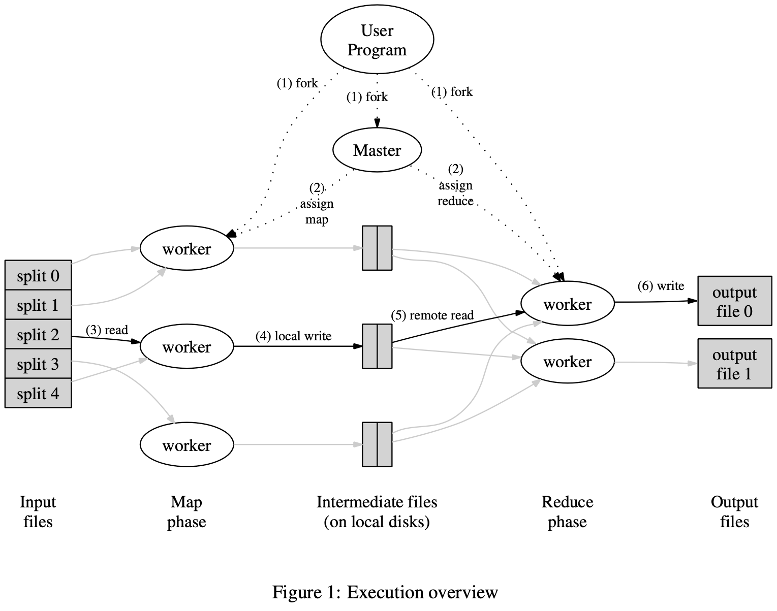
Figure 1 shows the overall flow of a MapReduce operation in our implementation. When the user program calls the MapReduce function, the following sequence of actions occurs (the numbered labels in Figure 1 correspond to the numbers in the list below):

Figure 1은 우리의 구현체에서의 MapReduce 작업의 전체 흐름을 보여줍니다. 사용자 프로그램이 MapReduce 함수를 호출하면 다음과 같은 순서로 작업이 이루어집니다(Figure 1의 번호 라벨은 아래 목록의 번호에 해당합니다).

The MapReduce library in the user program first splits the input files into M pieces of typically 16 megabytes to 64 megabytes (MB) per piece (controllable by the user via an optional parameter). It then starts up many copies of the program on a cluster of machines.

One of the copies of the program is special – the master. The rest are workers that are assigned work by the master. There are M map tasks and R reduce tasks to assign. The master picks idle workers and assigns each one a map task or a reduce task.

A worker who is assigned a map task reads the contents of the corresponding input split. It parses key/value pairs out of the input data and passes each pair to the user-defined Map function. The intermediate key/value pairs produced by the Map function are buffered in memory.

Periodically, the buffered pairs are written to local disk, partitioned into R regions by the partitioning function. The locations of these buffered pairs on the local disk are passed back to the master, who is responsible for forwarding these locations to the reduce workers.

When a reduce worker is notified by the master about these locations, it uses remote procedure calls to read the buffered data from the local disks of the map workers. When a reduce worker has read all intermediate data, it sorts it by the intermediate keys so that all occurrences of the same key are grouped together. The sorting is needed because typically many different keys map to the same reduce task. If the amount of intermediate data is too large to fit in memory, an external sort is used.

The reduce worker iterates over the sorted intermediate data and for each unique intermediate key encountered, it passes the key and the corresponding set of intermediate values to the user’s Reduce function. The output of the Reduce function is appended to a final output file for this reduce partition.

When all map tasks and reduce tasks have been completed, the master wakes up the user program. At this point, the MapReduce call in the user program returns back to the user code.

사용자 프로그램의 MapReduce 라이브러리는 먼저 입력 파일을 일반적으로 16MB ~ 64MB 크기를 갖는 M 개의 조각으로 나눕니다(크기는 사용자가 선택적 매개변수를 통해 제어 가능). 그런 다음 머신 클러스터에서 프로그램의 여러 복사본들을 실행하기 시작합니다.
프로그램 사본들 중 하나는 좀 특별한데, master 역할을 합니다. master가 아닌 나머지들은 master에 의해 작업을 할당받는 worker들입니다. 할당할 작업들로는 M개의 map 작업과 R개의 reduce 작업이 있습니다. master는 idle worker들을 선택하고 각각에게 map 작업 또는 reduce 작업을 할당합니다.
map 작업을 할당받은 worker는 해당하는 조각된 입력의 내용을 읽습니다. 그리고 입력 데이터에서 key/value 쌍을 파싱하고 각 쌍을 사용자 정의 Map 함수에 전달합니다. Map 함수에 의해 생성된 중간 key/value 쌍들은 메모리에 버퍼링됩니다.
주기적으로 버퍼링된 쌍이 로컬 디스크에 기록되고, 파티셔닝 함수에 의해 R개의 영역으로 나누어집니다. 로컬 디스크에 있는 이러한 버퍼링된 쌍들의 위치는 master에게 다시 전달되고, master는 이러한 위치들을 reduce worker들에게 전달하는 책임을 갖고 있습니다.
reduce worker가 master로부터 이러한 위치들에 대한 알림을 받게 되면, 원격 프로시저 호출을 사용하여 map worker의 로컬 디스크에 버퍼링된 데이터를 읽습니다. reduce worker가 모든 중간 데이터를 읽으면, 중간 key에 따라 데이터를 정렬하여 동일한 key의 모든 항목을 그루핑합니다. 이 때 정렬이 필요한데 일반적으로 서로 다른 많은 키들이 동일한 reduce 작업에 매핑되기 때문입니다. 중간 데이터의 양이 너무 커서 메모리에 들어갈 수 없는 경우라면 외부 정렬을 사용합니다.
reduce worker는 정렬된 중간 데이터를 순회하면서, 유니크한 중간 key가 발견될 때마다 해당 key와 해당 중간 value 집합을 사용자의 reduce 함수에 전달합니다. Reduce 함수의 출력은 이 reduce 파티션의 최종 출력 파일에 추가됩니다.
모든 map 작업과 reduce 작업이 완료되면, master는 사용자 프로그램을 깨웁니다. 이 시점에서 사용자 프로그램의 MapReduce 호출은 사용자 코드로 돌아갑니다.

After successful completion, the output of the mapreduce execution is available in the R output files (one per reduce task, with file names as specified by the user). Typically, users do not need to combine these R output files into one file – they often pass these files as input to another MapReduce call, or use them from another distributed application that is able to deal with input that is partitioned into multiple files.

모든 작업이 성공적으로 완료되면 mapreduce 실행의 출력 결과를 R개의 출력 파일(하나의 reduce 작업당 하나의 파일, 파일 이름은 사용자가 지정)을 통해 사용할 수 있게 됩니다. 일반적으로 사용자는 이러한 R 출력 파일을 하나의 파일로 결합할 필요가 없습니다. 보통은 이 파일들을 다른 MapReduce 호출의 입력으로 전달하거나, 여러 파일로 분할된 입력을 처리할 수 있는 다른 분산 애플리케이션에서 사용합니다.

3.2 Master Data Structures

Master 데이터 구조

The master keeps several data structures. For each map task and reduce task, it stores the state (idle, in-progress, or completed), and the identity of the worker machine (for non-idle tasks).

The master is the conduit through which the location of intermediate file regions is propagated from map tasks to reduce tasks. Therefore, for each completed map task, the master stores the locations and sizes of the R intermediate file regions produced by the map task. Updates to this location and size information are received as map tasks are completed. The information is pushed incrementally to workers that have in-progress reduce tasks.

master는 여러 데이터 구조를 유지합니다. 각 map 작업과 reduce 작업에 대해, 상태(idle, in-progress, completed)와 worker 머신의 식별자(idle 상태가 아닌 작업에 대해서)를 저장합니다.

master는 map 작업에서 reduce 작업으로 중간 파일 영역의 위치가 전달되는 통로이기도 합니다. 따라서 각 완료된 map 작업에 대해, master는 map 작업에 의해 생성된 R개의 중간 파일 영역의 위치와 크기를 저장합니다. map 작업이 완료될 때 이 위치와 크기 정보의 업데이트가 진행됩니다. 이 정보는 in-progress 상태인 reduce 작업을 갖고 있는 worker들에게 점진적으로 푸시됩니다.

3.3 Fault Tolernace

장애 허용성

Since the MapReduce library is designed to help process very large amounts of data using hundreds or thousands of machines, the library must tolerate machine failures gracefully.

MapReduce 라이브러리는 수백에서 수천 대의 머신을 사용하여 대규모의 데이터를 처리할 수 있도록 설계되었기 때문에, 머신의 장애를 우아하게 허용할 수 있어야 합니다.

Worker Failure

worker 장애

The master pings every worker periodically. If no response is received from a worker in a certain amount of time, the master marks the worker as failed. Any map tasks completed by the worker are reset back to their initial idle state, and therefore become eligible for scheduling on other workers. Similarly, any map task or reduce task in progress on a failed worker is also reset to idle and becomes eligible for rescheduling.

master는 주기적으로 모든 worker에게 ping을 보냅니다. 만약 특정 시간 내에 응답하지 못하는 worker가 있다면, master는 해당 worker를 실패한 것으로 표시합니다. 해당 worker가 완료한 모든 map 작업은 initial idle 상태로 재설정되므로, 다른 worker를 통해 스케줄링할 수 있게 됩니다.

Completed map tasks are re-executed on a failure because their output is stored on the local disk(s) of the failed machine and is therefore inaccessible. Completed reduce tasks do not need to be re-executed since their output is stored in a global file system.

실패한 워커가 완료시켜둔 map 작업은 해당 작업의 결과가 실패한 머신의 로컬 디스크에 저장되어 있어서 접근할 수 없기 때문에, 재실행됩니다. 완료된 reduce 작업은 전역 파일 시스템에 저장되어 있기 때문에 재실행할 필요가 없습니다.

When a map task is executed first by worker A and then later executed by worker B (because A failed), all workers executing reduce tasks are notified of the re-execution. Any reduce task that has not already read the data from worker A will read the data from worker B.

map 작업이 worker A에 의해 먼저 실행됐지만, (A가 실패했기 때문에) 나중에 worker B에 의해 실행되는 경우 reduce 작업을 실행하는 모든 worker들에게 작업 재실행 알림이 전송됩니다. worker A로부터의 데이터를 아직 읽지 않은 모든 reduce 작업은 worker B로부터의 데이터를 읽게 됩니다.

MapReduce is resilient to large-scale worker failures. For example, during one MapReduce operation, network maintenance on a running cluster was causing groups of 80 machines at a time to become unreachable for several minutes. The MapReduce master simply re-executed the work done by the unreachable worker machines, and continued to make forward progress, eventually completing the MapReduce operation.

MapReduce는 대규모의 worker 장애에 탄력적으로 대응할 수 있습니다. 예를 들어, 하나의 MapReduce 작업이 진행되는 동안, 실행 중인 클러스터에서 네트워크 유지보수가 수행되어 각 80대로 이루어진 여러 그룹의 머신들이 몇 분 동안 접근할 수 없게 된 적이 있었습니다. MapReduce master는 연결할 수 없게 된 worker 머신에서 수행하던 작업을 재실행하고 계속 진행해서 결국 MapReduce 작업을 완료했습니다.

Master Failure

master 장애

It is easy to make the master write periodic checkpoints of the master data structures described above. If the master task dies, a new copy can be started from the last checkpointed state. However, given that there is only a single master, its failure is unlikely; therefore our current implementation aborts the MapReduce computation if the master fails. Clients can check for this condition and retry the MapReduce operation if they desire.

master가 앞에서 설명한 master 데이터 구조에 대해 주기적인 체크포인트를 작성하게 하는 것은 쉽습니다. master 작업이 죽으면 마지막으로 체크포인트된 상태부터 새로운 복사본을 시작할 수 있습니다. 하지만 master가 단 하나뿐이기 때문에, master의 장애는 드뭅니다. 따라서 현재의 구현은 master가 실패하면 MapReduce 계산을 중단합니다. 클라이언트는 이런 상황을 인지하고, MapReduce 작업을 다시 시도할 수 있습니다.

Semantics in the Presence of Failures

장애가 발생했을 때의 의미론

When the user-supplied map and reduce operators are deterministic functions of their input values, our distributed implementation produces the same output as would have been produced by a non-faulting sequential execution of the entire program.

사용자가 제공한 map과 reduce 연산이 입력 값에 대한 결정론적인 함수라면, 우리의 분산 구현은 전체 프로그램을 오류 없이 순차적으로 실행했을 때와 동일한 출력을 생성합니다.

We rely on atomic commits of map and reduce task outputs to achieve this property. Each in-progress task writes its output to private temporary files. A reduce task produces one such file, and a map task produces R such files (one per reduce task). When a map task completes, the worker sends a message to the master and includes the names of the R temporary files in the message. If the master receives a completion message for an already completed map task, it ignores the message. Otherwise, it records the names of R files in a master data structure.

이러한 특성을 달성하기 위해 우리는 map과 reduce 작업의 출력을 원자적으로 커밋하도록 구현했습니다. 진행중인 각 작업들은 출력을 비공개 임시 파일에 기록합니다.

reduce 작업은 이런 파일을 하나 생성하고, map 작업은 R개의 파일을 생성합니다(reduce가 처리할 작업당 하나씩). map 작업이 완료되면 worker는 master에게 R 임시파일의 이름을 포함하고 있는 메시지를 보냅니다. master가 이미 완료된 map 작업에 대한 완료 메시지를 받으면, master는 메시지를 무시합니다. 그렇지 않으면, master는 R개의 파일의 이름을 master 데이터 구조에 기록합니다.

When a reduce task completes, the reduce worker atomically renames its temporary output file to the final output file. If the same reduce task is executed on multiple machines, multiple rename calls will be executed for the same final output file. We rely on the atomic rename operation provided by the underlying file system to guarantee that the final file system state contains just the data produced by one execution of the reduce task.

reduce 작업이 완료되면, reduce worker는 임시 출력 파일의 이름을 최종 출력 파일로 '원자적으로' 변경합니다. 만약 여러 머신에서 동일한 reduce 작업이 실행되면, 동일한 최종 출력 파일에 대해 여러 개의 rename 호출이 실행되게 됩니다. 우리는 최종 파일 시스템이 reduce 작업을 한 번 실행해 생성한 데이터만을 갖도록 하기 위해, 기반이 되는 파일 시스템이 제공하는 원자적인 rename 연산에 의존합니다.

The vast majority of our map and reduce operators are deterministic, and the fact that our semantics are equivalent to a sequential execution in this case makes it very easy for programmers to reason about their program’s behavior. When the map and/or reduce operators are non-deterministic, we provide weaker but still reasonable semantics. In the presence of non-deterministic operators, the output of a particular reduce task \(R_1\) is equivalent to the output for \(R_1\) produced by a sequential execution of the non-deterministic program. However, the output for a different reduce task \(R_2\) may correspond to the output for \(R_2\) produced by a different sequential execution of the non-deterministic program.

대부분의 map 과 reduce 연산은 결정론적이며, 그러한 경우 우리의 구현체의 의미론은 순차적 실행과 동일하기 때문에 프로그래머가 프로그램의 동작에 대해 추론하기 쉽습니다. map 또는 reduce 연산이 비결정론적인 경우에는 그보다는 약하지만 여전히 합리적인 의미론을 제공합니다. 비결정론적 연산이 있는 경우, 특정한 reduce 작업 \(R_1\)의 출력은 비결정론적 프로그램의 순차적 실행에 의해 생성된 \(R_1\)의 출력과 동일합니다. 그러나 다른 reduce 작업 \(R_2\)의 출력은 비결정론적 프로그램의 다른 순차적 실행에 의해 생성된 \(R_2\)의 출력과 일치하지 않을 수 있습니다.

Consider map task M and reduce tasks \(R_1\) and \(R_2\). Let \(e(R_i)\) be the execution of \(R_i\) that committed (there is exactly one such execution). The weaker semantics arise because \(e(R_1)\) may have read the output produced by one execution of M and \(e(R_2)\) may have read the output produced by a different execution of M.

예를 들어 map 작업 M과, reduce 작업 \(R_1\), \(R_2\)가 있다고 생각해 봅시다. 작업 \(R_i\)가 실행되어 이미 커밋된 것을 \(e(R_i)\)라고 합시다(이렇게 커밋된 실행은 단 하나만 있을 수 있습니다). 앞에서 언급한 '약한 의미론'은, \(e(R_1)\)이 M의 실행 결과 중 하나를 읽었지만, \(e(R_2)\)가 M의 다른 실행 결과를 읽을 수 있기 때문에 발생합니다.

3.4 Locality

지역성

Network bandwidth is a relatively scarce resource in our computing environment. We conserve network bandwidth by taking advantage of the fact that the input data (managed by GFS [8]) is stored on the local disks of the machines that make up our cluster. GFS divides each file into 64 MB blocks, and stores several copies of each block (typically 3 copies) on different machines. The MapReduce master takes the location information of the input files into account and attempts to schedule a map task on a machine that contains a replica of the corresponding input data. Failing that, it attempts to schedule a map task near a replica of that task’s input data (e.g., on a worker machine that is on the same network switch as the machine containing the data). When running large MapReduce operations on a significant fraction of the workers in a cluster, most input data is read locally and consumes no network bandwidth.

네트워크 대역폭은 우리의 컴퓨팅 환경에서 상대적으로 부족한 자원입니다. 우리는 클러스터를 구성하는 머신의 로컬 디스크에 입력 데이터(GFS [8]로 관리함)가 저장된다는 사실을 활용하여 네트워크 대역폭을 절약합니다. GFS는 각각의 파일들을 64MB 짜리 블록으로 나눠서, 각 블록의 복사본들(보통 3개)을 서로 다른 컴퓨터에 저장합니다. MapReduce master는 입력 파일의 위치 정보를 고려하여, 해당 입력 데이터의 복사본을 포함하고 있는 머신에 대해 map 작업을 예약하려 시도합니다. 이 예약이 실패하면 해당 작업의 입력 데이터 복제본 근처(예: 데이터를 갖고 있는 머신과 동일한 네트워크 스위치에 있는 다른 worker 머신)에서 map 작업의 예약을 시도합니다. 클러스터를 이루는 상당수의 worker들에 대해 대규모 MapReduce 작업을 실행하게 되면, 대부분의 입력 데이터는 로컬로 읽혀지므로 네트워크 대역폭을 소비하지 않습니다.

3.5 Task Granularity

작업의 단위

We subdivide the map phase into M pieces and the reduce phase into R pieces, as described above. Ideally, M and R should be much larger than the number of worker machines. Having each worker perform many different tasks improves dynamic load balancing, and also speeds up recovery when a worker fails: the many map tasks it has completed can be spread out across all the other worker machines.

앞에서 설명한 바와 같이 map 단계는 M개의 작업으로, reduce 단계는 R개의 작업으로 나누게 됩니다. 이상적으로는, M과 R은 worker 머신의 수보다 훨씬 큰 값이어야 합니다. 각 worker가 여러 작업을 수행하게 하면 동적 로드 밸런싱이 향상되며, worker에 장애가 발생했을 경우에도 복구 속도가 빨라집니다. worker가 완료한 많은 map 작업을 다른 모든 worker 머신에 분산시킬 수 있기 때문입니다.

There are practical bounds on how large M and R can be in our implementation, since the master must make \(O(M + R)\) scheduling decisions and keeps \(O(M ∗ R)\) state in memory as described above. (The constant factors for memory usage are small however: the \(O(M ∗ R)\) piece of the state consists of approximately one byte of data per map task/reduce task pair.)

앞에서 설명한 바와 같이 master는 \(O(M + R)\) 스케쥴링 결정을 내리고, \(O(M ∗ R)\) 상태를 메모리에 유지해야 하므로, M과 R이 얼마나 커질 수 있는지에 대해서는 실제 구현에서는 한계가 있습니다. (그러나 메모리 사용량에 대해서 상수 조건은 작은 편입니다. \(O(M ∗ R)\) 상태의 일부는 map 작업/reduce 작업 쌍 당 약 1바이트의 데이터로 구성됩니다.)

Furthermore, R is often constrained by users because the output of each reduce task ends up in a separate output file. In practice, we tend to choose M so that each individual task is roughly 16 MB to 64 MB of input data (so that the locality optimization described above is most effective), and we make R a small multiple of the number of worker machines we expect to use. We often perform MapReduce computations with M = 200, 000 and R = 5, 000, using 2,000 worker machines.

또한, 각 reduce 작업의 출력은 별도의 출력 파일에 저장되기 때문에, R은 종종 사용자에 의한 제약을 받곤 합니다. 실제로는 위에서 이야기한 지역 최적화가 가장 효과를 발휘할 수 있도록, 각 개별 작업의 입력 데이터가 대략적으로 16MB ~ 64MB가 되드록 M을 선택하고, 사용할 worker 머신 수의 크지 않은 배수로 R을 설정하는 경향이 있습니다. 우리는 종종 2000대의 worker 머신을 사용하여 M = 200,000, R = 5,000으로 MapReduce 계산을 수행합니다.

3.6 Backup Tasks

백업 작업

One of the common causes that lengthens the total time taken for a MapReduce operation is a “straggler”: a machine that takes an unusually long time to complete one of the last few map or reduce tasks in the computation. Stragglers can arise for a whole host of reasons. For example, a machine with a bad disk may experience frequent correctable errors that slow its read performance from 30 MB/s to 1 MB/s. The cluster scheduling system may have scheduled other tasks on the machine, causing it to execute the MapReduce code more slowly due to competition for CPU, memory, local disk, or network bandwidth. A recent problem we experienced was a bug in machine initialization code that caused processor caches to be disabled: computations on affected machines slowed down by over a factor of one hundred.

MapReduce 작업에 소요되는 전체 시간을 늘리는 일반적인 원인 중 하나는 "straggler"(지연자)입니다. 지연자란 계산의 마지막 몇 개의 map 또는 reduce 작업 중 하나를 완료하는 데에 비정상적으로 오랜 시간이 걸리는 머신을 말합니다. 지연자가 발생하는 이유는 다양합니다. 예를 들어, 불량한 디스크를 갖고 있는 머신은 오류가 자주 발생해서 읽기 성능이 30MB/s 내지 1MB/s 정도로 느려지기도 합니다. 클러스터 스케쥴링 시스템이 특정한 머신에 다른 작업을 예약한다던가 해서 CPU, 메모리, 로컬 디스크 또는 네트워크 대역폭에 대한 경쟁이 발생해 MapReduce 코드를 더 느리게 실행하게 될 수도 있습니다. 우리가 최근에 경험한 문제 하나는 머신 초기화 코드에 버그가 있어서 프로세서 캐시가 비활성화되는 것이었는데, 이 문제의 영향을 받은 머신에서의 계산은 100배 이상 느려졌습니다.

We have a general mechanism to alleviate the problem of stragglers. When a MapReduce operation is close to completion, the master schedules backup executions of the remaining in-progress tasks. The task is marked as completed whenever either the primary or the backup execution completes. We have tuned this mechanism so that it typically increases the computational resources used by the operation by no more than a few percent. We have found that this significantly reduces the time to complete large MapReduce operations. As an example, the sort program described in Section 5.3 takes 44% longer to complete when the backup task mechanism is disabled.

우리에게는 지연자 발생 문제를 완화하기 위한 일반적인 메커니즘이 있습니다. MapReduce 작업이 거의 완료됐을 때, master는 진행중 상태인 나머지 작업들의 백업 실행을 예약합니다. 기본적인 실행이나 백업 실행이 완료될 때마다 작업은 완료된 것으로 표시됩니다. 이 메커니즘을 통해 일반적으로 작업에 사용되는 컴퓨팅 리소스는 몇 퍼센트 이상 증가시키지 않도록 조정됐습니다. 예를 들어, 5.3절에서 설명하는 정렬 프로그램에서 백업 작업 메커니즘을 비활성화하면 완료하기까지 44% 더 많은 시간이 걸리게 됩니다.

확장 기능들

Although the basic functionality provided by simply writing Map and Reduce functions is sufficient for most needs, we have found a few extensions useful. These are described in this section.

Map과 Reduce 함수를 작성하는 것만으로도 대부분의 요구사항을 충분히 만족시킬 수 있지만, 우리는 몇 가지 확장 기능들이 유용하다는 것을 발견했습니다.

4.1 Partitioning Function

파티셔닝 함수

The users of MapReduce specify the number of reduce tasks/output files that they desire (R). Data gets partitioned across these tasks using a partitioning function on the intermediate key. A default partitioning function is provided that uses hashing (e.g. “hash(key) mod R”). This tends to result in fairly well-balanced partitions. In some cases, however, it is useful to partition data by some other function of the key. For example, sometimes the output keys are URLs, and we want all entries for a single host to end up in the same output file. To support situations like this, the user of the MapReduce library can provide a special partitioning function. For example, using “hash(Hostname(urlkey)) mod R” as the partitioning function causes all URLs from the same host to end up in the same output file.

MapReduce의 사용자가 reduce 작업/출력 파일의 수(R)를 자신이 원하는 값으로 지정하면, 데이터는 중간 key의 파티셔닝 함수를 통해서 그러한 작업들에 분할됩니다. 이 때 기본으로 제공되는 파티셔닝 함수는 해싱을 사용합니다(예: "hash(key) mod R"). 이 함수를 사용하면 꽤 균형 잡힌 파티션이 만들어집니다. 그러나 경우에 따라서는 데이터를 파티셔닝할 때 용도에 따라 다른 함수를 key에 사용하는 것이 유용할 때도 있습니다. 예를 들어, 출력 key가 URL인 경우가 있습니다. 이때는 같은 호스트에 대한 모든 항목이 동일한 출력 파일에 저장되도록 하고 싶을 수 있습니다. 이러한 상황을 지원하려면, MapReduce 라이브러리의 사용자는 특별한 파티셔닝 함수를 제공하면 됩니다. 예를 들어, 파티셔닝 함수로 "hash(Hostname(urlkey)) mod R"을 사용하면 동일한 호스트의 모든 URL이 동일한 출력 파일에 저장되는 것입니다.

4.2 Ordering Guarantees

순서 보장

We guarantee that within a given partition, the intermediate key/value pairs are processed in increasing key order. This ordering guarantee makes it easy to generate a sorted output file per partition, which is useful when the output file format needs to support efficient random access lookups by key, or users of the output find it convenient to have the data sorted.

우리는 주어진 파티션 내에서 중간 key/value 쌍에 대해 처리되는 key가 오름차순으로 처리된다는 것을 보장합니다.

이러한 순서 보장을 통해 파티션별로 정렬된 출력 파일을 쉽게 생성할 수 있습니다. 이런 특징은 key에 대한 효율적인 랜덤 액세스 조회가 필요한 출력 결과가 필요하거나 출력 결과의 사용자에게 데이터가 정렬되어 있는 것이 편리한 경우에 유용합니다.

4.3 Combiner Function

조합 함수

In some cases, there is significant repetition in the intermediate keys produced by each map task, and the userspecified Reduce function is commutative and associative. A good example of this is the word counting example in Section 2.1. Since word frequencies tend to follow a Zipf distribution, each map task will produce hundreds or thousands of records of the form <the, 1>. All of these counts will be sent over the network to a single reduce task and then added together by the Reduce function to produce one number. We allow the user to specify an optional Combiner function that does partial merging of this data before it is sent over the network.

The Combiner function is executed on each machine that performs a map task. Typically the same code is used to implement both the combiner and the reduce functions. The only difference between a reduce function and a combiner function is how the MapReduce library handles the output of the function. The output of a reduce function is written to the final output file. The output of a combiner function is written to an intermediate file that will be sent to a reduce task.

Partial combining significantly speeds up certain classes of MapReduce operations. Appendix A contains an example that uses a combiner.

어떤 경우에는, 각각의 map 작업에서 생성되는 중간 key들에 중복이 많이 발생하면서 사용자가 교환법칙과 결합법칙을 만족하는 Reduce 함수를 지정하는 상황이 있습니다. 2.1절의 단어 카운팅 예제가 이에 해당하는 사례라 할 수 있습니다. 단어 빈도는 일반적으로 [[/jargon/zipf-s-law]]{Zipf 분포}를 따르므로 각 map 작업은 <the, 1> 형태의 수백, 수천 개의 레코드를 생성합니다. 이러한 모든 카운트는 네트워크를 통해 하나의 reduce 작업으로 전송되며, Reduce 함수를 통해 합산되어 하나의 숫자가 됩니다. 이런 경우, 네트워크를 통해 전송되기 전의 데이터를 부분적으로 병합하는 선택적인 combiner 함수를 사용자가 지정할 수 있습니다.

combiner 함수는 map 작업을 수행하는 각 머신에서 실행됩니다. 일반적으로 combiner 함수와 reduce 함수의 구현에는 똑같은 코드가 사용됩니다. reduce 함수와 combiner 함수의 차이점은 MapReduce 라이브러리가 함수의 출력을 어떻게 처리하는지 뿐입니다. reduce 함수의 출력은 최종 출력 파일에 쓰여지는 반면, combiner 함수의 출력은 reduce 작업으로 전송될 중간 파일에 쓰여지는 것입니다.

부분적인 조합은 MapReduce 작업의 특정 유형을 매우 빠르게 만들어 줄 수 있습니다. 부록 A에 combiner를 사용하는 예제가 포함되어 있습니다.

4.4 Input and Output Types

입력과 출력의 유형

The MapReduce library provides support for reading input data in several different formats. For example, “text” mode input treats each line as a key/value pair: the key is the offset in the file and the value is the contents of the line. Another common supported format stores a sequence of key/value pairs sorted by key. Each input type implementation knows how to split itself into meaningful ranges for processing as separate map tasks (e.g. text mode’s range splitting ensures that range splits occur only at line boundaries). Users can add support for a new input type by providing an implementation of a simple reader interface, though most users just use one of a small number of predefined input types.

MapReduce 라이브러리는 여러가지 다양한 포맷의 입력 데이터를 읽을 수 있습니다. 예를 들어, "text"모드 입력은 각 라인을 key/value 쌍으로 취급합니다. 이렇게 읽는 경우 key는 파일의 offset이 되고, value는 각 라인의 내용이 됩니다. MapReduce 라이브러리가 지원하는 또다른 일반적인 포맷은 key를 기준으로 정렬된 key/value 쌍의 시퀀스를 저장하는 포맷입니다. 각각의 입력 타입 구현에는 별도의 map 작업으로 처리할 수 있도록 의미있는 범위로 나누는 방법이 포함되어 있습니다. (예: text 모드의 범위 쪼개기는 범위 분할이 라인 경계에서만 발생하도록 보장합니다.) 사용자는 간단한 reader 인터페이스 구현을 제공하는 방식으로 새로운 입력 타입에 대한 지원을 추가할 수 있지만, 대부분의 사용자들은 미리 정의된 몇 개의 입력 타입들 중 하나를 사용하곤 합니다.

A reader does not necessarily need to provide data read from a file. For example, it is easy to define a reader that reads records from a database, or from data structures mapped in memory.

In a similar fashion, we support a set of output types for producing data in different formats and it is easy for user code to add support for new output types.

reader가 꼭 파일을 통해서만 데이터를 읽어야 하는 것은 아닙니다. 예를 들어, 데이터베이스나 인메모리에 매핑된 자료구조에서 레코드를 읽는 reader를 정의하는 것은 쉬운 일입니다.

이와 비슷한 방식으로, 다양한 포맷의 데이터를 생성하기 위한 출력 타입 집합을 지원합니다. 그리고 사용자 코드를 통해 새로운 출력 타입을 추가하는 것도 쉽습니다.

4.5 Side-effects

부수 효과

In some cases, users of MapReduce have found it convenient to produce auxiliary files as additional outputs from their map and/or reduce operators. We rely on the application writer to make such side-effects atomic and idempotent. Typically the application writes to a temporary file and atomically renames this file once it has been fully generated.

We do not provide support for atomic two-phase commits of multiple output files produced by a single task. Therefore, tasks that produce multiple output files with cross-file consistency requirements should be deterministic. This restriction has never been an issue in practice.

MapReduce의 사용자들 중 몇몇은 경우에 따라 map이나 reduce 연산의 추가적인 출력을 통해 부가적인 파일을 생성하는 것이 편리하다는 것을 알게 됐습니다. 우리는 이러한 부수 효과가 원자성과 멱등성을 갖도록 하는 것은 애플리케이션 작성자에게 의존하기로 했습니다. 일반적으로 애플리케이션은 기록을 임시 파일에 하고, 임시 파일이 완전히 생성되면 파일 이름을 원자적으로 변경합니다.

단일 작업을 통해 생성된 여러 출력 파일에 대해서는 원자적인 2단계 커밋을 지원하지 않습니다. 따라서, 여러 출력 파일에 걸친 일관성 요구 사항을 가진 작업은 결정론적인 특징을 갖고 있어야 합니다. 이런 제약 사항은 실제 활용 상황에서는 문제가 된 적이 없습니다.

4.6 Skipping Bad Records

나쁜 레코드 건너뛰기

Sometimes there are bugs in user code that cause the Map or Reduce functions to crash deterministically on certain records. Such bugs prevent a MapReduce operation from completing. The usual course of action is to fix the bug, but sometimes this is not feasible; perhaps the bug is in a third-party library for which source code is unavailable. Also, sometimes it is acceptable to ignore a few records, for example when doing statistical analysis on a large data set. We provide an optional mode of execution where the MapReduce library detects which records cause deterministic crashes and skips these records in order to make forward progress.

사용자 코드로 제공된 Map이나 Reduce 함수에 버그가 있어서 특정 레코드에 대해 결정론적으로 작업이 실패하는 경우가 있습니다. 이런 버그 때문에 MapReduce 작업이 완료되지 못할 수 있습니다. 이 문제에 대한 일반적인 조치는 버그를 수정하는 것이지만, 소스코드가 제공되지 않는 서드 파티 라이브러리에 버그가 있는 경우라면 이런 조치를 취할 수 없습니다. 또한, 대용량 데이터셋에 대한 통계 분석을 수행하는 경우와 같이 몇몇 레코드를 무시하는 것이 필요한 경우도 있습니다. 우리는 MapReduce 라이브러리가 어떤 레코드가 결정론적인 실패를 유발하는지 감지하고, 이런 레코드를 건너뛰어서 전진할 수 있도록 선택적 실행 모드를 제공합니다.

Each worker process installs a signal handler that catches segmentation violations and bus errors. Before invoking a user Map or Reduce operation, the MapReduce library stores the sequence number of the argument in a global variable. If the user code generates a signal, the signal handler sends a “last gasp” UDP packet that contains the sequence number to the MapReduce master. When the master has seen more than one failure on a particular record, it indicates that the record should be skipped when it issues the next re-execution of the corresponding Map or Reduce task.

각각의 worker 프로세스는 세그멘테이션 위반과 버스 에러를 잡아내는 시그널 핸들러를 설치합니다. 사용자 Map이나 Reduce 연산을 호출하기 전에, MapReduce 라이브러리는 인자의 시퀀스 번호를 전역 변수에 저장합니다. 만약 사용자 코드가 시그널을 생성한다면, 시그널 핸들러는 시퀀스 번호를 포함하는 "마지막 호흡" UDP 패킷을 MapReduce 마스터에게 전송합니다. 만약 마스터가 특정 레코드에 대해 하나 이상의 실패를 발견했다면, 이는 해당 레코드가 다음 Map이나 Reduce 작업을 재실행할 때 건너뛰어져야 한다는 것을 의미합니다.

4.7 Local Execution

로컬 실행

Debugging problems in Map or Reduce functions can be tricky, since the actual computation happens in a distributed system, often on several thousand machines, with work assignment decisions made dynamically by the master. To help facilitate debugging, profiling, and small-scale testing, we have developed an alternative implementation of the MapReduce library that sequentially executes all of the work for a MapReduce operation on the local machine. Controls are provided to the user so that the computation can be limited to particular map tasks. Users invoke their program with a special flag and can then easily use any debugging or testing tools they find useful (e.g. gdb).

Map이나 Reduce 함수를 디버깅하는 것은 까다로운 일입니다. 실제 계산이 수천대의 머신으로 분산된 시스템에서 이루어지는 상황에서, 마스터가 동적으로 작업 할당을 하기 때문입니다. 디버깅, 프로파일링, 소규모의 테스팅을 용이하게 하기 위해, 우리는 로컬 머신에서 모든 작업을 순차적으로 실행하는 방식의 MapReduce 대체 구현체를 개발했습니다. 특정 map 작업에 대해서만 계산을 제한할 수 있도록 사용자에게 컨트롤이 제공되는 것이 특징입니다. 사용자는 특수한 플래그를 사용하여 프로그램을 호출하고, 그 후에는 디버깅이나 테스팅에 적합한 도구를 간편하게 사용할 수 있습니다. (예: gdb)

4.8 Status Information

상태 정보

The master runs an internal HTTP server and exports a set of status pages for human consumption. The status pages show the progress of the computation, such as how many tasks have been completed, how many are in progress, bytes of input, bytes of intermediate data, bytes of output, processing rates, etc. The pages also contain links to the standard error and standard output files generated by each task. The user can use this data to predict how long the computation will take, and whether or not more resources should be added to the computation. These pages can also be used to figure out when the computation is much slower than expected.

In addition, the top-level status page shows which workers have failed, and which map and reduce tasks they were processing when they failed. This information is useful when attempting to diagnose bugs in the user code.

master는 내부적으로 HTTP 서버를 가동하며, 사람이 알아볼 수 있는 상태정보 페이지를 제공합니다. 상태정보 페이지에서는 완료된 작업의 수, 진행중인 작업의 수, 입력된 바이트의 양, 중간 데이터 바이트의 양, 출력 바이트의 양, 처리된 비율 등의 계산 진행 정보를 보여줍니다. 이 페이지에는 각 작업에서 생성된 표준 에러와 표준 출력 파일로의 링크도 포함되어 있습니다. 사용자는 이 데이터를 통해 계산이 얼마나 걸릴지, 계산에 얼마나 더 많은 리소스가 필요한지를 예측할 수 있습니다. 이런 페이지들은 계산이 예상보다 훨씬 느리게 진행되고 있는지를 파악하는데도 사용될 수 있습니다.

또한, 최상위 상태정보 페이지에서는 어떤 worker가 실패했는지, 실패한 worker가 어떤 map과 reduce 작업을 처리하고 있었는지를 보여줍니다. 이 정보는 사용자 코드의 버그를 진단하는 데 유용합니다.

4.9 Counters

카운터

The MapReduce library provides a counter facility to count occurrences of various events. For example, user code may want to count total number of words processed or the number of German documents indexed, etc.

MapReduce 라이브러리는 다양한 이벤트의 발생 횟수를 세는 카운터 기능을 제공합니다. 예를 들어 사용자 코드는 처리된 단어의 총 개수라던가, 인덱싱된 독일어 문서의 개수 등을 세는 것이 필요할 수도 있습니다.

To use this facility, user code creates a named counter object and then increments the counter appropriately in the Map and/or Reduce function. For example:

이 기능을 사용하려면 사용자 코드는 카운터 객체를 생성한 다음, Map이나 Reduce 함수에서 적절하게 카운터를 증가시키면 됩니다. 예를 들자면 다음과 같습니다.

Counter* uppercase;
uppercase = GetCounter("uppercase");

map(String name, String contents):
  for each word w in contents:
    if (IsCapitalized(w)):
      uppercase->Increment();
    EmitIntermediate(w, "1");

The counter values from individual worker machines are periodically propagated to the master (piggybacked on the ping response). The master aggregates the counter values from successful map and reduce tasks and returns them to the user code when the MapReduce operation is completed. The current counter values are also displayed on the master status page so that a human can watch the progress of the live computation. When aggregating counter values, the master eliminates the effects of duplicate executions of the same map or reduce task to avoid double counting. (Duplicate executions can arise from our use of backup tasks and from re-execution of tasks due to failures.)

각 worker 머신에서 집계한 카운터 값은 주기적으로 master로 전달됩니다(ping 응답에 함께 전달). master는 성공한 map과 reduce 작업의 카운터 값을 집계하고, MapReduce 작업이 완료되면 집계한 값을 사용자 코드로 리턴합니다. 이 대, 현재의 카운터 값은 master 상태 페이지에서도 표시되므로, 사람이 실시간으로 계산의 진행 상황을 확인할 수 있습니다. 카운터 값을 집계할 때, master는 동일한 map이나 reduce 작업의 중복 실행 효과를 제거하여 중복 계산을 방지합니다. (백업 작업이나, 실패로 인한 재실행 때문에 중복 실행이 발생할 수 있습니다.)

Some counter values are automatically maintained by the MapReduce library, such as the number of input key/value pairs processed and the number of output key/value pairs produced.

MapReduce 라이브러리에 의해 자동으로 관리되는 카운터 종류도 몇 가지 있습니다. 예를 들어 처리된 입력 키/값 쌍의 개수나, 생성된 출력 키/값 쌍의 개수 등이 이에 해당합니다.

Users have found the counter facility useful for sanity checking the behavior of MapReduce operations. For example, in some MapReduce operations, the user code may want to ensure that the number of output pairs produced exactly equals the number of input pairs processed, or that the fraction of German documents processed is within some tolerable fraction of the total number of documents processed.

사용자들은 MapReduce 작업의 동작을 검증하는 용도로도 카운터 기능이 유용하다고 생각하게 됐습니다. 예를 들어, 어떤 MapReduce 작업에서는 사용자 코드가 생성된 출력 쌍의 개수가 정확히 입력 쌍의 개수와 같은지를 확인하거나, 처리된 독일어 문서의 비율이 처리된 전체 문서의 비율로 보면 어느 정도인지를 확인하고 싶을 수 있습니다.

5 Performance

성능

In this section we measure the performance of MapReduce on two computations running on a large cluster of machines. One computation searches through approximately one terabyte of data looking for a particular pattern. The other computation sorts approximately one terabyte of data.

이번 섹션에서 우리는 대규모 머신 클러스터에서 실행되는 두 가지 계산에 대한 MapReduce의 성능을 측정합니다. 첫 번째 계산은 약 1TB의 데이터에서 특정 패턴을 검색해 찾는 것이고, 두 번째 계산은 약 1TB의 데이터를 정렬하는 것입니다.

These two programs are representative of a large subset of the real programs written by users of MapReduce – one class of programs shuffles data from one representation to another, and another class extracts a small amount of interesting data from a large data set.

이 두 계산 프로그램은 MapReduce 사용자들이 실제로 작성하는 프로그램들의 대부분을 대표한다고 볼 수 있습니다. 하나는 데이터의 표현 방식을 다른 표현으로 바꾸는 작업을 하고, 다른 하나는 대용량 데이터 세트에서 흥미로운 데이터를 추출하는 것입니다.

5.1 Cluster Configuration

클러스터 구성

All of the programs were executed on a cluster that consisted of approximately 1800 machines. Each machine had two 2GHz Intel Xeon processors with Hyper-Threading enabled, 4GB of memory, two 160GB IDE disks, and a gigabit Ethernet link. The machines were arranged in a two-level tree-shaped switched network with approximately 100-200 Gbps of aggregate band-width available at the root. All of the machines were in the same hosting facility and therefore the round-trip time between any pair of machines was less than a millisecond.

모든 프로그램은 약 1800대의 머신으로 구성된 클러스터에서 실행되었습니다. 각 머신은 2GHz Intel Xeon 프로세서 2개를 장착하고 있으며, Hyper-Threading이 활성화되어 있고, 4GB의 메모리, 160GB의 IDE 디스크 2개, 그리고 기가비트 이더넷 링크를 가지고 있습니다. 머신들은 2레벨 트리 구조의 스위치 네트워크에 배치되었으며, 해당 네트워크는 루트 기준으로 약 100-200Gbps의 대역폭을 갖추고 있습니다. 모든 머신은 동일한 호스팅 시설에 있었기 때문에, 모든 두 머신 간의 왕복 시간은 1ms 미만이었습니다.

Out of the 4GB of memory, approximately 1-1.5GB was reserved by other tasks running on the cluster. The programs were executed on a weekend afternoon, when the CPUs, disks, and network were mostly idle.

4GB의 메모리 중 약 1-1.5GB는 클러스터에서 실행되는 다른 작업들을 위해 예약되어 있습니다. 프로그램들은 CPU, 디스크, 네트워크가 대부분 유휴 상태인 주말 오후에 실행되었습니다.

5.2 Grep

grep

The grep program scans through 10¹⁰ 100-byte records, searching for a relatively rare three-character pattern (the pattern occurs in 92,337 records). The input is split into approximately 64MB pieces (M = 15000), and the entire output is placed in one file (R = 1).

Figure 2 shows the progress of the computation over time. The Y-axis shows the rate at which the input data is scanned. The rate gradually picks up as more machines are assigned to this MapReduce computation, and peaks at over 30 GB/s when 1764 workers have been assigned. As the map tasks finish, the rate starts dropping and hits zero about 80 seconds into the computation. The entire computation takes approximately 150 seconds from start to finish. This includes about a minute of startup overhead. The overhead is due to the propagation of the program to all worker machines, and delays interacting with GFS to open the set of 1000 input files and to get the information needed for the locality optimization.

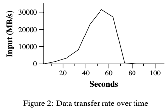
grep 프로그램은 100byte로 이루어진 레코드 10¹⁰개를 스캔하여, 드물게 나타나는 세 글자로 이루어진 패턴을 찾습니다(총 92,337개의 레코드에서 이 패턴을 찾아야 합니다). 입력은 약 64MB 크기의 조각으로 쪼개지며(M = 15000), 전체 출력은 하나의 파일로 저장됩니다(R = 1).

Figure 2는 시간에 따른 계산 진행 상황을 보여줍니다. Y축은 입력 데이터의 스캔 속도를 보여줍니다. 입력 데이터의 스캔 속도는 더 많은 머신이 MapReduce 계산에 할당되면서 점차 늘어나고, 1764개의 worker가 할당되었을 때 30GB/s 이상이 되어 최고치를 찍습니다. map 작업이 끝나면 속도는 다시 떨어지며, 계산이 시작된 후 80초가 지났을 때 0이 됩니다. 전체 계산은 시작부터 끝까지 약 150초가 소요되며, 여기에는 약 1분 정도의 시작 오버헤드가 포함됩니다. 오버헤드는 프로그램이 모든 worker 머신에 전파되는 데 필요한 시간과, 1000개의 입력 파일을 열고 로컬리티 최적화를 위해 필요한 정보를 GFS로부터 가져오는 데 필요한 시간 때문에 발생합니다.

5.3 Sort

sort

The sort program sorts 10¹⁰ 100-byte records (approximately 1 terabyte of data). This program is modeled after the TeraSort benchmark [10].

sort 프로그램은 100byte로 이루어진 레코드 10¹⁰개(약 1TB의 데이터)를 정렬합니다. 이 프로그램은 TeraSort 벤치마크[10]를 참고해 만든 것입니다.

The sorting program consists of less than 50 lines of user code. A three-line Map function extracts a 10-byte sorting key from a text line and emits the key and the original text line as the intermediate key/value pair. We used a built-in Identity function as the Reduce operator. This functions passes the intermediate key/value pair unchanged as the output key/value pair. The final sorted output is written to a set of 2-way replicated GFS files (i.e., 2 terabytes are written as the output of the program).

이 sort 프로그램은 50줄 미만의 사용자 코드로 이루어져 있습니다. 3줄짜리 Map 함수가 텍스트 한 줄에서 10byte의 정렬 키를 추출하고, 추출한 키와 해당 텍스트 라인을 중간 키/값 쌍으로 출력하는 방식입니다. 우리는 Reduce 연산자로 빌트인 Identity 함수를 선택해 사용했습니다. Identity 함수는 넘겨받은 중간 키/값 쌍을 변경 없이 그대로 출력 키/값 쌍으로 전달하는 것입니다. 최종 정렬된 결과는 2-way로 복제된 GFS 파일들에 쓰여집니다(즉, 2TB가 프로그램의 출력 기록으로 사용됩니다).

As before, the input data is split into 64MB pieces (M = 15000). We partition the sorted output into 4000 files (R = 4000). The partitioning function uses the initial bytes of the key to segregate it into one of R pieces.

이전과 마찬가지로 입력 데이터는 64MB 크기의 조각으로 나눠집니다(M = 15000). 그리고 정렬된 출력 결과는 4000개의 파일로 분할됩니다(R = 4000). 파티셔닝 함수는 key의 초기 바이트를 기준으로 해당 키를 R개의 조각 중 하나로 분배합니다.

Our partitioning function for this benchmark has built-in knowledge of the distribution of keys. In a general sorting program, we would add a pre-pass MapReduce operation that would collect a sample of the keys and use the distribution of the sampled keys to compute split-points for the final sorting pass.

이 벤치마크에 사용된 우리의 파티셔닝 함수는 key의 분포에 대한 정보를 내장하고 있습니다. 일반적인 정렬 프로그램에서는, 키 샘플을 수집하는 사전 패스 MapReduce 작업을 추가합니다. 이는 샘플 키의 분포를 참고하여 최종 정렬 단계의 분할 지점을 계산하기 위해서입니다.

Figure 3 (a) shows the progress of a normal execution of the sort program. The top-left graph shows the rate at which input is read. The rate peaks at about 13 GB/s and dies off fairly quickly since all map tasks finish before 200 seconds have elapsed. Note that the input rate is less than for grep. This is because the sort map tasks spend about half their time and I/O bandwidth writing intermediate output to their local disks. The corresponding intermediate output for grep had negligible size.

Figure 3 (a)는 sort 프로그램이 정상적으로 실행되는 과정을 보여줍니다. 왼쪽 열 상단의 그래프는 입력이 읽히는 속도를 보여줍니다. 이 속도는 약 13GB/s에서 최고치를 찍고나서 200초 이내에 모든 Map 작업이 완료되기 때문에 상당히 빠르게 감소합니다. grep과 비교했을 때 입력 속도가 더 낮다는 점에 주목해야 합니다. 이는 sort Map 작업이 절반 정도의 시간과 I/O 대역폭을 사용하여 중간 결과를 로컬 디스크에 기록하기 때문입니다. 반면, grep의 경우 중간 출력의 크기가 무시할 만큼 작았습니다.

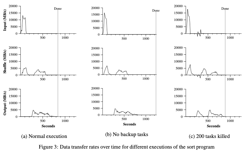
The middle-left graph shows the rate at which data is sent over the network from the map tasks to the reduce tasks. This shuffling starts as soon as the first map task completes. The first hump in the graph is for the first batch of approximately 1700 reduce tasks (the entire MapReduce was assigned about 1700 machines, and each machine executes at most one reduce task at a time). Roughly 300 seconds into the computation, some of these first batch of reduce tasks finish and we start shuffling data for the remaining reduce tasks. All of the shuffling is done about 600 seconds into the computation.

왼쪽 열 중간에 있는 그래프는 Map 작업에서 Reduce 작업으로 데이터가 네트워크를 통해 전송되는 속도를 보여줍니다. 이 셔플링은 첫 번째 Map 작업이 완료되자마자 시작됩니다. 그래프에서 처음 나타나는 봉우리 모양은 약 1700개의 Reduce 작업의 첫 번째 배치를 나타냅니다(전체 MapReduce는 약 1700대의 머신에 할당되었고, 각 머신은 한 번에 최대 하나의 Reduce 작업을 실행합니다). 계산이 시작된 지 약 300초가 지났을 때, 이 첫 번째 배치의 Reduce 작업 중 일부가 완료되고, 그 다음에 남은 Reduce 작업에 대한 데이터 셔플링이 시작됩니다. 모든 셔플링은 계산 시작으로부터 약 600초 후에 완료됩니다.

The bottom-left graph shows the rate at which sorted data is written to the final output files by the reduce tasks. There is a delay between the end of the first shuffling period and the start of the writing period because the machines are busy sorting the intermediate data. The writes continue at a rate of about 2-4 GB/s for a while. All of the writes finish about 850 seconds into the computation. Including startup overhead, the entire computation takes 891 seconds. This is similar to the current best reported result of 1057 seconds for the TeraSort benchmark [18].

왼쪽 열 아래의 그래프는 reduce 작업으로 정렬된 데이터가 최종 출력 파일에 기록되는 속도를 보여줍니다. 머신들이 중간 데이터를 정렬하느라 바쁘기 때문에, 첫 번째 셔플링 기간이 끝나고 나서 쓰기가 시작될 때까지 지연 시간이 좀 발생하게 됩니다. 쓰기는 약 2-4GB/s의 속도로 계속되다가, 계산 시작으로부터 약 850초가 지난 후에 모든 쓰기가 완료됩니다. 시작 오버헤드를 포함하면 전체 계산은 891초가 걸립니다. 이는 TeraSort 벤치마크의 현재 최고 기록인 1057초와 비슷한 결과입니다.

A few things to note: the input rate is higher than the shuffle rate and the output rate because of our locality optimization – most data is read from a local disk and bypasses our relatively bandwidth constrained network. The shuffle rate is higher than the output rate because the output phase writes two copies of the sorted data (we make two replicas of the output for reliability and availability reasons). We write two replicas because that is the mechanism for reliability and availability provided by our underlying file system. Network bandwidth requirements for writing data would be reduced if the underlying file system used erasure coding [14] rather than replication.

다음의 몇 가지 사항에 유의해야 합니다:

로컬 최적화로 인해 입력 속도가 셔플 속도와 출력 속도보다 높습니다. 대부분의 데이터를 로컬 디스크에서 읽기 때문에 상대적으로 대역폭이 제한되는 네트워크를 우회하게 됩니다. 셔플 속도가 출력 속도보다 높은 이유는 출력 단계에서 정렬된 데이터를 두 개의 복사본으로 기록하기 때문입니다(우리는 신뢰성과 가용성을 위해 출력에 대해 두 개의 사본을 만듭니다). 두 개의 사본을 만드는 이유는 이 방법이 우리의 기본 파일 시스템이 신뢰성과 가용성을 제공하는 메커니즘이기 때문입니다. 기본 파일 시스템이 복제가 아니라 삭제 코딩[14]을 사용한다면 데이터를 기록하기 위한 네트워크 대역폭 요구 사항이 줄어들 것입니다.

5.4 Effect of Backup Tasks

백업 작업의 영향

In Figure 3 (b), we show an execution of the sort program with backup tasks disabled. The execution flow is similar to that shown in Figure 3 (a), except that there is a very long tail where hardly any write activity occurs. After 960 seconds, all except 5 of the reduce tasks are completed. However these last few stragglers don’t finish until 300 seconds later. The entire computation takes 1283 seconds, an increase of 44% in elapsed time.

Figure 3 (b)는 백업 작업이 비활성화된 상태에서 sort 프로그램이 실행되는 과정을 보여줍니다. 실행 흐름은 Figure 3 (a)에 나타난 것과 거의 비슷하나, 꽤 긴 시간동안 쓰기 활동이 거의 없는 상황이 발생한다는 차이점이 있습니다. 960초가 지나면 reduce 작업 중 5개를 제외한 모든 작업이 완료됩니다. 하지만 그 이후 이 마지막 몇 개의 작업은 300초가 지난 후에야 완료됩니다. 전체 계산에 1283초가 소요되며, 이는 경과 시간이 44% 증가한 것을 의미합니다.

5.5 Machine Failures

머신 실패

In Figure 3 (c), we show an execution of the sort program where we intentionally killed 200 out of 1746 worker processes several minutes into the computation. The underlying cluster scheduler immediately restarted new worker processes on these machines (since only the processes were killed, the machines were still functioning properly).

Figure 3 (c)는 sort 프로그램의 실행을 보여줍니다. 이 실행에서는 계산이 시작된 지 몇 분 후에 1746개의 worker 프로세스 중 200개를 의도적으로 종료시켰습니다. 기본 클러스터 스케줄러는 이 머신들에 대해 즉시 새로운 worker 프로세스를 재시작합니다(프로세스만 종료되었기 때문에 머신은 여전히 정상적으로 작동하고 있었습니다).

The worker deaths show up as a negative input rate since some previously completed map work disappears (since the corresponding map workers were killed) and needs to be redone. The re-execution of this map work happens relatively quickly. The entire computation finishes in 933 seconds including startup overhead (just an increase of 5% over the normal execution time).

worker 프로세스의 종료로 인해 이전에 완료된 일부 map 작업이 유실되어(map worker들이 kill됐기 때문) 다시 수행되어야 하기 때문에, 입력 속도가 마이너스로 표시됩니다. 이 map 작업의 재실행은 비교적 빠르게 이루어집니다. 시작 오버헤드를 포함하면 전체 계산은 933초만에 완료되며, 이는 일반적인 실행 시간보다 5%만 증가한 것입니다.

6 Experience

We wrote the first version of the MapReduce library in February of 2003, and made significant enhancements to it in August of 2003, including the locality optimization, dynamic load balancing of task execution across worker machines, etc. Since that time, we have been pleasantly surprised at how broadly applicable the MapReduce library has been for the kinds of problems we work on. It has been used across a wide range of domains within Google, including:

우리는 2003년 2월에 MapReduce 라이브러리의 첫 번째 버전을 작성했습니다. 그리고 2003년 8월에는 로컬 최적화, worker 머신들 간 작업 실행의 동적 로드 밸런싱 등 라이브러리를 크게 개선했습니다. 그 후, 우리는 MapReduce 라이브러리가 우리가 다루는 문제들에 대해 얼마나 광범위하게 적용될 수 있는지에 대해 놀라움을 느끼게 됐습니다. 이 라이브러리는 Google의 다양한 도메인에서 활용되었습니다.

large-scale machine learning problems,

clustering problems for the Google News and Froogle products,

extraction of data used to produce reports of popular queries (e.g. Google Zeitgeist),

extraction of properties of web pages for new experiments and products (e.g. extraction of geographical locations from a large corpus of web pages for localized search), and

large-scale graph computations.

대규모의 머신 러닝 문제,
Google 뉴스와 Froogle 제품의 클러스터링 문제,
인기 검색어에 대한 보고서를 생성하기 위해 사용되는 데이터 추출하기(예: Google Zeitgeist),
새로운 실험과 제품을 위한 웹 페이지의 속성 추출하기(예: 지역화된 검색을 위한 대량의 웹 페이지 코퍼스에서 지리적 위치 추출),
대규모의 그래프 계산

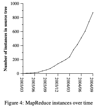
Figure 4 shows the significant growth in the number of separate MapReduce programs checked into our primary source code management system over time, from 0 in early 2003 to almost 900 separate instances as of late September 2004. MapReduce has been so successful because it makes it possible to write a simple program and run it efficiently on a thousand machines in the course of half an hour, greatly speeding up the development and prototyping cycle. Furthermore, it allows programmers who have no experience with distributed and/or parallel systems to exploit large amounts of resources easily.

Figure 4는 주요 소스 코드 관리 시스템에 체크인된 별도의 MapReduce 프로그램의 수의 변화를 보여줍니다. MapReduce 프로그램은 2003년 초에는 0개였지만 시간이 지남에 따라 크게 증가하여 2004년 9월 말에는 거의 900개에 달하게 되었습니다. MapReduce는 꽤나 성공적이었는데, 간단한 프로그램을 작성하면 30분 동안 1000개의 머신에서 효율적으로 실행할 수 있어, 개발 및 프로토타이핑 주기를 크게 단축시킬 수 있었기 때문입니다. 또한 분산 및 병렬 시스템에 대한 경험이 없는 프로그래머들이 쉽게 많은 리소스를 활용할 수 있도록 해주었습니다.

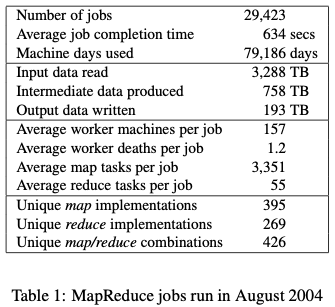
At the end of each job, the MapReduce library logs statistics about the computational resources used by the job. In Table 1, we show some statistics for a subset of MapReduce jobs run at Google in August 2004.

각 작업이 끝날 때마다 MapReduce 라이브러리는 작업에서 사용한 계산 리소스에 대한 통계를 기록합니다. Table 1은 2004년 8월에 Google에서 실행된 MapReduce 작업에 대한 통계를 보여줍니다.

table 1

6.1 Large-Scale Indexing

대규모 인덱싱

One of our most significant uses of MapReduce to date has been a complete rewrite of the production indexing system that produces the data structures used for the Google web search service. The indexing system takes as input a large set of documents that have been retrieved by our crawling system, stored as a set of GFS files. The raw contents for these documents are more than 20 terabytes of data. The indexing process runs as a sequence of five to ten MapReduce operations. Using MapReduce (instead of the ad-hoc distributed passes in the prior version of the indexing system) has provided several benefits:

Google 웹 검색 서비스에 사용되는 데이터 구조를 생성하는 프로덕션 인덱싱 시스템을 완전히 재개발하는 것은 지금까지 MapReduce를 사용한 사례들 중 가장 중요한 것이라 할 수 있습니다. 인덱싱 시스템은 크롤링 시스템에 의해 검색된 대량의 문서들을 입력으로 받아 GFS 파일의 집합으로 저장합니다. 이러한 문서들의 원시 컨텐츠의 용량은 20TB 이상의 데이터에 달합니다. 인덱싱 프로세스는 5개에서 10개의 MapReduce 작업으로 구성됩니다. 인덱싱 시스템의 이전 버전에서 사용된 ad-hoc 분산 패스 대신 MapReduce를 사용하면 다음과 같은 이점이 있습니다.

The indexing code is simpler, smaller, and easier to understand, because the code that deals with fault tolerance, distribution and parallelization is hidden within the MapReduce library. For example, the size of one phase of the computation dropped from approximately 3800 lines of C++ code to approximately 700 lines when expressed using MapReduce.

The performance of the MapReduce library is good enough that we can keep conceptually unrelated computations separate, instead of mixing them together to avoid extra passes over the data. This makes it easy to change the indexing process. For example, one change that took a few months to make in our old indexing system took only a few days to implement in the new system.

The indexing process has become much easier to operate, because most of the problems caused by machine failures, slow machines, and networking hiccups are dealt with automatically by the MapReduce library without operator intervention. Furthermore, it is easy to improve the performance of the indexing process by adding new machines to the indexing cluster.

내결함성을 보장하고 분산처리 및 병렬화를 처리하는 코드가 MapReduce 라이브러리 내부에 숨겨져 있기 때문에, 인덱싱 코드가 더 간단하고 작아서 이해하기 쉽습니다. 예를 들어, 특정 단계의 계산에서 3800줄의 C++ 코드가 MapReduce를 사용하여 표현하면 약 700줄로 줄어들었습니다.
MapReduce 라이브러리의 성능이 충분히 좋기 때문에, 데이터를 여러 번 읽는 것을 피하게 하려고 개념적으로 관련이 없는 계산을 잡다하게 섞어서 사용하는 것을 하지 않아도 됩니다. 이로 인해 인덱싱 프로세스를 쉽게 변경할 수 있습니다. 예를 들어, 이전 인덱싱 시스템에서 몇 달이 걸렸던 변경 작업이 새 시스템에서는 며칠 만에 구현할 수 있었습니다.
머신 장애, 느린 머신, 네트워킹 딸꾹질(간헐적 장애)로 인해 발생하는 대부분의 문제가 운영자가 개입하지 않아도 MapReduce 라이브러리가 알아서 자동으로 처리하기 때문에 인덱싱 프로세스를 훨씬 더 쉽게 운영할 수 있게 됐습니다. 또한, 인덱싱 클러스터에 새로운 머신을 추가해서 인덱싱 프로세스의 성능을 쉽게 개선할 수 있습니다.

8 Conclusions

결론

The MapReduce programming model has been successfully used at Google for many different purposes. We attribute this success to several reasons. First, the model is easy to use, even for programmers without experience with parallel and distributed systems, since it hides the details of parallelization, fault-tolerance, locality optimization, and load balancing. Second, a large variety of problems are easily expressible as MapReduce computations. For example, MapReduce is used for the generation of data for Google’s production web search service, for sorting, for data mining, for machine learning, and many other systems. Third, we have developed an implementation of MapReduce that scales to large clusters of machines comprising thousands of machines. The implementation makes efficient use of these machine resources and therefore is suitable for use on many of the large computational problems encountered at Google.

Google에서는 MapReduce 프로그래밍 모델을 다양한 목적으로 성공적으로 사용하고 있습니다. 이러한 성공에는 몇 가지 이유가 있습니다.

첫째, 사용하기 쉽습니다.
- 병렬화, 장애 처리, 로컬 최적화, 부하 분산 등의 세부 사항을 숨기기 때문에 병렬 및 분산 시스템에 대한 경험이 없는 프로그래머도 쉽게 사용할 수 있는 모델입니다.
둘째, 다양한 문제를 MapReduce 계산으로 쉽게 표현할 수 있습니다.
- 예를 들어 MapReduce는 Google의 제품 웹 검색 서비스의 데이터 생성, 정렬, 데이터 마이닝, 기계 학습 등에 사용됩니다.
셋째, 우리는 수천 대의 머신으로 구성된 대규모 머신 클러스터로 확장할 수 있는 MapReduce 구현을 개발해냈습니다.
- 이 구현은 이러한 머신 리소스를 효율적으로 사용하므로 Google에서 직면하는 많은 대규모 계산 문제에 사용하기에 적합합니다.

We have learned several things from this work. First, restricting the programming model makes it easy to parallelize and distribute computations and to make such computations fault-tolerant. Second, network bandwidth is a scarce resource. A number of optimizations in our system are therefore targeted at reducing the amount of data sent across the network: the locality optimization allows us to read data from local disks, and writing a single copy of the intermediate data to local disk saves network bandwidth. Third, redundant execution can be used to reduce the impact of slow machines, and to handle machine failures and data loss.

우리는 MapReduce 작업을 통해 몇 가지 배운 것들이 있습니다.

첫째, 프로그래밍 모델을 제한하면 계산을 병렬화하고 분산화하는 등의 계산을 쉽게 만들 수 있고, 이러한 계산이 내결함성을 갖도록 만들 수 있습니다.
둘째, 네트워크 대역폭은 희소한 자원입니다.
- 따라서 우리 시스템의 최적화는 네트워크를 통해 전송되는 데이터의 양을 줄이는 데 초점을 맞추고 있습니다. 로컬 최적화를 통해 로컬 디스크에서 데이터를 읽을 수 있고, 중간 데이터의 단일 복사본을 디스크에 쓰는 방식으로 네트워크 대역폭을 절약할 수 있습니다.
셋째, 중복 실행을 활용하면 느린 머신으로 인한 영향을 줄일 수 있으며, 머신 장애나 데이터 손실과 같은 문제도 처리할 수 있습니다.

Acknowledgments

감사의 말

Josh Levenberg has been instrumental in revising and extending the user-level MapReduce API with a number of new features based on his experience with using MapReduce and other people’s suggestions for enhancements. MapReduce reads its input from and writes its output to the Google File System [8]. We would like to thank Mohit Aron, Howard Gobioff, Markus Gutschke, David Kramer, Shun-Tak Leung, and Josh Redstone for their work in developing GFS. We would also like to thank Percy Liang and Olcan Sercinoglu for their work in developing the cluster management system used by MapReduce. Mike Burrows, Wilson Hsieh, Josh Levenberg, Sharon Perl, Rob Pike, and Debby Wallach provided helpful comments on earlier drafts of this paper. The anonymous OSDI reviewers, and our shepherd, Eric Brewer, provided many useful suggestions of areas where the paper could be improved. Finally, we thank all the users of MapReduce within Google’s engineering organization for providing helpful feedback, suggestions, and bug reports.

Josh Levenberg는 MapReduce 사용 경험과 다른 사람들의 개선 제안을 바탕으로 여러 가지 새로운 기능으로 사용자 수준의 MapReduce API를 수정하고 확장하는 데 중요한 역할을 해왔습니다. MapReduce는 Google File System[8]에서 입력을 읽고 출력을 씁니다. GFS를 개발해 주신 Mohit Aron, Howard Gobioff, Markus Gutschke, David Kramer, Shun-Tak Leung, Josh Redstone에게 감사의 말씀을 전합니다. 또한 MapReduce에서 사용하는 클러스터 관리 시스템을 개발해 주신 Percy Liang과 Olcan Sercinoglu에게도 감사의 말씀을 전합니다. Mike Burrows, Wilson Hsieh, Josh Levenberg, Sharon Perl, Rob Pike, Debby Wallach이 이 논문의 초기 초안에 대해 유용한 의견을 제공해 주셨습니다. 익명의 OSDI 검토자들과 우리의 논문 지도자(shepherd)인 Eric Brewer는 논문을 개선할 수 있는 유용한 제안을 많이 해주셨습니다. 마지막으로, 유용한 피드백, 제안, 버그 리포트를 제공해 주신 Google 엔지니어링 조직 내의 모든 MapReduce 사용자에게 감사드립니다.

References

참고문헌

[1] Andrea C. Arpaci-Dusseau, Remzi H. Arpaci-Dusseau, David E. Culler, Joseph M. Hellerstein, and David A. Patterson. High-performance sorting on networks of workstations. In Proceedings of the 1997 ACM SIGMOD International Conference on Management of Data, Tucson, Arizona, May 1997.
[2] Remzi H. Arpaci-Dusseau, Eric Anderson, Noah Treuhaft, David E. Culler, Joseph M. Hellerstein, David Patterson, and Kathy Yelick. Cluster I/O with River: Making the fast case common. In Proceedings of the Sixth Workshop on Input/Output in Parallel and Distributed Systems (IOPADS ’99), pages 10–22, Atlanta, Georgia, May 1999.
[3] Arash Baratloo, Mehmet Karaul, Zvi Kedem, and Peter Wyckoff. Charlotte: Metacomputing on the web. In Proceedings of the 9th International Conference on Parallel and Distributed Computing Systems, 1996.
[4] Luiz A. Barroso, Jeffrey Dean, and Urs Hölzle. Web search for a planet: The Google cluster architecture. IEEE Micro, 23(2):22–28, April 2003.
[5] John Bent, Douglas Thain, Andrea C.Arpaci-Dusseau, Remzi H. Arpaci-Dusseau, and Miron Livny. Explicit control in a batch-aware distributed file system. In Proceedings of the 1st USENIX Symposium on Networked Systems Design and Implementation NSDI, March 2004.
[6] Guy E. Blelloch. Scans as primitive parallel operations. IEEE Transactions on Computers, C-38(11), November 1989.
[7] Armando Fox, Steven D. Gribble, Yatin Chawathe, Eric A. Brewer, and Paul Gauthier. Cluster-based scalable network services. In Proceedings of the 16th ACM Symposium on Operating System Principles, pages 78– 91, Saint-Malo, France, 1997.
[8] Sanjay Ghemawat, Howard Gobioff, and Shun-Tak Leung. The Google file system. In 19th Symposium on Operating Systems Principles, pages 29–43, Lake George, New York, 2003.
[9] S. Gorlatch. Systematic efficient parallelization of scan and other list homomorphisms. In L. Bouge, P. Fraigniaud, A. Mignotte, and Y. Robert, editors, Euro-Par’96. Parallel Processing, Lecture Notes in Computer Science 1124, pages 401–408. Springer-Verlag, 1996.
[10] Jim Gray. Sort benchmark home page. http://research.microsoft.com/barc/SortBenchmark/.
[11] William Gropp, Ewing Lusk, and Anthony Skjellum. Using MPI: Portable Parallel Programming with the Message-Passing Interface. MIT Press, Cambridge, MA, 1999.
[12] L. Huston, R. Sukthankar, R. Wickremesinghe, M. Satyanarayanan, G. R. Ganger, E. Riedel, and A. Ailamaki. Diamond: A storage architecture for early discard in interactive search. In Proceedings of the 2004 USENIX File and Storage Technologies FAST Conference, April 2004.
[13] Richard E. Ladner and Michael J. Fischer. Parallel prefix computation. Journal of the ACM, 27(4):831–838, 1980.
[14] Michael O. Rabin. Efficient dispersal of information for security, load balancing and fault tolerance. Journal of the ACM, 36(2):335–348, 1989.
[15] Erik Riedel, Christos Faloutsos, Garth A. Gibson, and David Nagle. Active disks for large-scale data processing. IEEE Computer, pages 68–74, June 2001.
[16] Douglas Thain, Todd Tannenbaum, and Miron Livny. Distributed computing in practice: The Condor experience. Concurrency and Computation: Practice and Experience, 2004.
[17] L. G. Valiant. A bridging model for parallel computation. Communications of the ACM, 33(8):103–111, 1997.
[18] Jim Wyllie. Spsort: How to sort a terabyte quickly. http://alme1.almaden.ibm.com/cs/spsort.pdf.

A Word Frequency

단어 빈도 구하기

This section contains a program that counts the number of occurrences of each unique word in a set of input files specified on the command line.

이 섹션에는 커맨드 라인으로 지정된 입력 파일 집합에서 각 고유한 단어의 발생 횟수를 세는 프로그램이 포함되어 있습니다.

소스 코드 생략.

주석

MPI는 Message-Passing Interface를 의미하며, MPI primitives는 MPI에서 정의하는 기본적인 함수나 연산들을 말한다. ↩

번역